This component generates a step function. It is initialized by the following three parameters:

Step Time: the time at which the output signal changes;

Initial Value: the value of the signal prior to the step change;

Final Value: the signal's value following the step change.

This component creates a sine wave of the form

and so takes three parameters:

Amplitude: the value of A;

Frequency: the value of w ;

Phase: the value of f .

This element generates a linear transfer function of the form

.

Note that the denominator's order must be greater than or equal to that of the numerator (i.e., n ³ m). This component takes two parameters:

Numerator: an array containing the coefficients of the numerator's polynomial, descending from the highest order in s (i.e., a_m, a_m-1, ...);

Denominator: an array containing the coefficients of the denominator's polynomial, descending from the highest order in s (i.e., b_m, b_m-1, ...).

This element simulates an ideal PID controller with transfer function

.

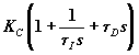It takes the following three parameters:

P: the steady-state gain, K_C,

I: equivalent to K_C/t _I;

D: equivalent to K_{Ct D}.

This element multiplies the input by an amount K_P, i.e.,

It takes one parameter:

Gain: the value of K_P.

Note that Gain can consist of a constant or variable. Further, the input x can be either a scalar quantity or a vector.

This element delays the input signal by a given amount of time. It is therefore particularly useful when a transportation lag is needed. Two parameters are required:

Time Delay: the lag time,

Initial Input: the output signal from the component at start of the simulation until the time equals the lag period. This typically is 0.

This component limits the range of an output signal to within prescribed upper and lower bounds. If the input signal exceeds this range, the output is clipped to the bounding value. The Saturation element is therefore useful for including physical limits on components such as valves and for studying reset windup. It takes two parameters:

Lower Limit: the lower limit of the output signal,

Upper Limit: the signal's upper limit.

The Sum connection adds or subtracts various signals to yield a net signal. It is therefore used to create summers and comparators in control loops. The Sum component takes a single parameter:

List of Signs: a string of + and - signs, for example, + + - - + .

The number of inputs to the element is determined by the number of signs in the string. The sense of the input (i.e., positive or negative) is determined by the sign itself. For example, + + + sums three input signals together to produce a single output. The string +- , meanwhile, creates a comparator that subtracts one signal from another.

The Demux element separates a vector signal into scalar signals. It takes one parameter:

Number of Outports: the number of scalar signals leaving the device.

The Mux element carries out the inverse operation of the Demux ¾ it combines scalar signals into a vector signal. It also takes a single parameter:

Number of Inports: the number of scalar signals entering the device.

The Mux element can be used to generate an output array that contains the time and output from the control loop as columns in the matrix. These can then be sent to the MATLAB workspace using the To Workspace component described later.

This element provides interactive plotting of data as a function of simulation time. It includes five key parameters:

Initial Time Range: the initial length of the t axis (this axis adjusts as the simulation proceeds),

Initial Y Min: the initial lower limit on the y axis (this adjusts as the simulation proceeds),

Initial Y Max: the initial upper limit on the y axis (this adjusts as the simulation proceeds),

Storage Points: the number of data points retained in the curve,

Sample Time: determines the rate of data acquisition for plotting purposes.

The Clock element provides a means for recording the simulation time for later use in calculations. This feature is particularly useful if one intends to send the output signal to the MATLAB workspace for further analysis.

This component creates a matrix containing data from a vector input signal and writes it to the MATLAB workspace. It takes two parameters:

Variable Name: the name of the MATLAB matrix containing the data,

Max # of Rows (timesteps): gives the number of rows of the matrix (each column in the matrix will contain rows holding the signal value at the corresponding time step in the simulation).