MCG 3341 FLUID MECHANICS II - Professor S. Tavoularis
COMPUTATIONAL ASSIGNMENT
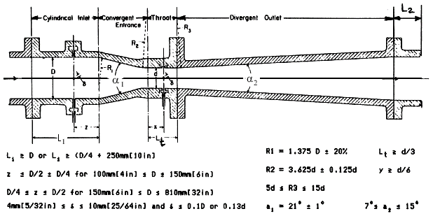
ASME STANDARD VENTURI TUBE SPECIFICATIONS

Reference: Measurement of Fluid Flow in Pipes Using Orifice, Nozzle and Venturi, ASME MFC-3M-1985, Amer. Soc. Mech. Eng.,1985.
Specifications for All Students:
D = 10 mm, a1 = 21 deg, a2 = 14 deg, L1/D = 15,
L2/D = 5, Lt/D = 1;
use only straight lines for the contour (do not round corners)
fluid: water at 20 deg C
inlet flow: uniform flow, with a speed V
Reynolds number: Re = r V D /
m , where r, m are, respectively, density and viscosity
Note: Specifications of lengths, velocities and material properties in Star-CCM+ are dimensionl. Make sure to specify all values in the correct units and compute the velocity value such as to obtain the specified Re.
Individual Specifications:
Student number: auvwxyz (if your number has six digits, let a = 0)
d/D = vw %, if v = 4, 5, 6 or 7 (for example, if v = 4 and w = 5, then
d/D = 45%)
d/D = (v + 4)x %, if v = 0, 1, 2 or 3 (for example, if v = 3 and x = 0, then d/D = 70%)
d/D = (v - 2)y %, if v = 8 or 9 (for example, if v = 9 and y = 3, d/D=73%)
1. a) (Marks: 10%) Provide the following:
Notes: Provide zoomed detail plots of appropriate flow regions, especially at the inlet and near locations of area change. Adjust the aspect ratio of each plot (i.e., use different scales for radial and axial axes), so that all information presented is clearly visible and not too crowded.
2. (Marks: 20%) Conduct a mesh dependence study by repeating the computations for three different meshes, the finest of which has at least 5 times more elements than the coarsest one and is as fine as your computer memory allows. Compare the results of the three computations quantitatively (i.e., percent differences) for values of velocity and pressure at selected locations. Also compare the computational times required by each computation.
3. (Marks: 20%) Repeat the computation, as in Part 1, increasing the Reynolds number to the highest value that produces a solution. Adjust the mesh as necessary. Provide plots as in Part 1, including zoomed plots.
4. (Marks: 20%) Discuss all results obtained in Parts 1, 2 and 3. In particular,
N.B.: Present your assignment in the style of a technical report. Divide the material in chapters (and sections, if required), including a brief introduction and conclusions. Make sure to number all pages and figures and to provide figure captions.
Total Marks: 100%
1. (Marks: 70%) Consider the Venturi tube with the same general and personal specifications as for the laminar flow. Compute the steady, axisymmetric, turbulent flow through the Venturi tube at the largest Reynolds number that produces a solution (see instructions for turbulent flow and for higher Reynolds number). Provide the following plots:
Note: Provide zoomed detail plots of appropriate flow regions, especially at the inlet and near locations of area change.
2. (Marks: 30%) Discuss all results obtained in Part 1. In particular,
N.B.: Present your assignment in the style of a technical report. Divide the material in chapters (and sections, if required), including a brief introduction and conclusions. Make sure to number all pages and figures and to provide figure captions.
Total Marks: 100%
TIPS FOR COMPUTATIONS RAM (Random Access Memory) : While you run a simulation, you can monitor the system's RAM consumption using the System Monitor tool that comes with Windows. Grids with smaller mesh sizes (or, equivalently, higher mesh densities) will consume more RAM. It is a good idea to note how much RAM your simulation is consuming. This will allow you to gauge how small you can make your grid size.
Units: Make sure that your units are consistentfor all geometrical and material
parameters.
TROUBLESHOOTING
For troubleshooting consult the User Guide located in the Help menu under Tutorial Guide. This will open up documentation in a new browser. Look for User Guide on the left of the window.
Start with the program that you used for laminar flow computation. Save it as a new program with a different filename and keep the original program for future reference. You need to make a few modifications in order to compute turbulent flows. The process is relatively straightforward and explained in the following paragraphs. For more information on running turbulent simulations see the Tutorial Guide (Introduction Tutorial) that comes with Star-CCM+. See Getting Started with Star-CCM+ for more information on accessing the tutorials. The main changes required are as follows.
CREATE A NEW PHYSICS MODEL
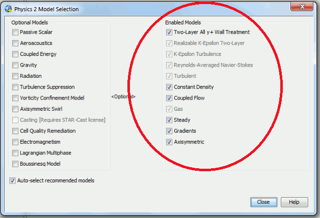
Right click on the Continua node and click New > Physics Continuum. On the new Physics model that appears under the Continua node, click Select Models (up to now this is the same process as for Laminar Flows). In the window that appears be sure to check the following options: Axisymmetric, Steady, Gas, Coupled Flow, Constant Density, Turbulent, and K-Epsilon Turbulence. This is a common and relatively simple turbulence model. k is the turbulent kinetic energy per unit mass, which is an
indication of the intensity of the turbulent fluctuations. k has the dimension
of velocity square, so that the square root of k is a velocity scale of
turbulence. The turbulent kinetic energy is continuously being dissipated into
heat, i.e., the relative velocity differences between eddies diminish by being converted to random molecular motions.
This process is called turbulent energy dissipation and epsilon is the rate of dissipation of k. The ratio k/epsilon has dimensions of
time and can be considered as a time scale of turbulence. Your window should then look like the image below:


 and convert to 2D, following instructions in the Tutorial. Note, you will have to clear your solution before running your new simulation. You will also have to re-create your scenes for the new solution.
Don't forget to save all changes in a new file by selecting Save As in the File menu.
STRATEGIES FOR PERFORMING COMPUTATIONS AT HIGH REYNOLDS NUMBERS
REFINING THE MESH
To improve your solution, the mesh should be refined in areas of rapidly changing
geometry. Also, each element should have a good aspect ratio, which is the ratio
of the lengths of the longest to the shortest side of an element. Try to create
elements that are as square as possible (a ratio of the shortest edge to the
longest edge of up to 2 or 3 is acceptable, but if you go above that you may
compromise the quality of the solution.)
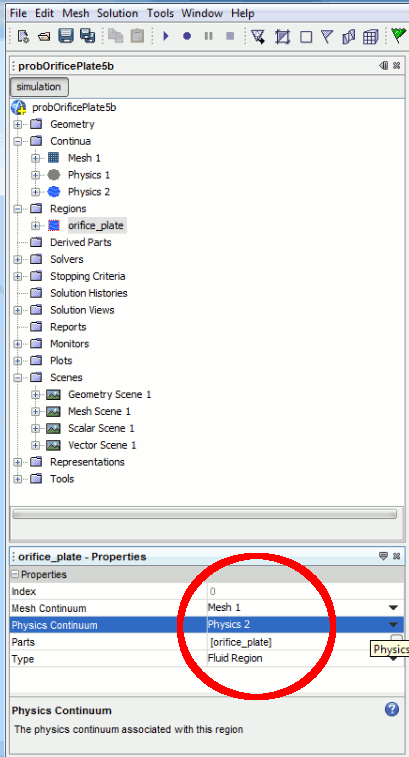
To refine your mesh, or change your grid type, you will have to first regenerate it in 3D and convert it to 2D. First, it is highly recommended that you Save As.. a different filename before proceeding. Once you change your grid parameters under the Continua > Mesh 1 node, you will need to delete any 2D physics and regions you have previously generated. To do this, right click on the appropriate 2D node under Continua or Regions and click Delete. Next, ensure that your 3D region is pointing to the correct Mesh and 3D Physics. Now, regenerate the mesh with the Generate Volume Mesh Button
INCREASING THE NUMBER OF ITERATIONS ALLOWED
The solution in Star-CCM+ is solved using an iterative solver. The solver iterates
at each time step until the residuals (i.e., differences between the solution
values at each iteration and those at the previous iteration) become smaller
than a certain value. The default number of iterations for Star-CCM+ is 1000. You can
change this number to allow for more or less iterations. Increasing this does not always produce a solution,
because the residuals may not necessarily decrease after a few iterations, but
fluctuate about relatively large values. To change the number of iterations,
open the Stopping Criteria > Maximum Steps node and find the Maximum Steps value in the properties window. Do not make this too large, as the program will waste a lot of
time iterating for a solution that may not converge.
INCREASING THE INLET VELOCITY (i.e., THE REYNOLDS NUMBER)
To increase the inlet velocity, you will have to change the inlet boundary condition. To do this, open the Regions > assignment_region 2D > Boundaries > Inlet > Physics Values > Velocity Magnitude > Constant node and set the Value to correspond to the Reynolds number you wish to compute. Note that your region may have a different name, depending on how you named it in the first place. Remember to clear your solution before running the simulation at the new Reynolds number. Increase the Reynolds number by a factor of 10 each time using this process until you find that the solution does not converge (remember that, for convergence, all residuals should tend to zero). In your final repo, report only the details of the solution for the highest Reynolds number that converged, but also describe briefly what happened when you tried to sol;ve the problem for higher Re.
 and convert it to 2D, following instructions in the Tutorial. Note, you will have to clear your solution before running your new simulation. You will also have to re-create your scenes for the new solution.